Adaptive-Dimensional Block-Sparse Featurizers:
Learning How Wide Each Concept Should Be

Edward Lu

Research notes · August 2026 · not peer reviewed · combined write-up: BSF beyond fixed widths · related: semantic-aligned BSF

Abstract Block-sparse featurizers (Fel et al., 2026) give every concept a block of fixed, hand-chosen width b. We make the width learnable: ordered prefix gates let each block choose its own dimension under a dimension-use penalty, with block Top-K sparsity untouched. On the paper's controlled synthetic toy model the gates recover how many concepts exist and how wide each one is; with a gate warm-up the adaptive model beats every fixed-width control across seeds, and a shuffled-width control shows the win comes from which concept gets which width. On DINOv2 features the same mechanism keeps 276 of 4,096 blocks yet nearly matches a raw-feature probe, an unsupervised filter that keeps task-useful structure.

1Problem: fixed width is wrong for most concepts

BSF blocks hold multi-dimensional concepts together: a circle wants 2 dimensions, a sphere 3, instead of shattering them across rank-one atoms.
But b is one global hand-set choice. On the paper's own toy model true concept widths span 1–3, so any single b over-provisions the 1-D segments and can starve wider manifolds. The paper resolves this by sweeping b.
Question: can the featurizer allocate width by itself: learning both whether a block should exist and how many dimensions it deserves?

2Method: ordered prefix gates

Each block gets a maximum width b_max and gate logits θ. Soft mask = cumulative product of sigmoids, so it only decreases along dimensions, the hard mask is always a prefix: 1,1,1,0,0,0 → width 3.
Forward pass uses the hard {0,1} mask with a straight-through gradient: turned off dimensions are exactly inactive, not merely small.
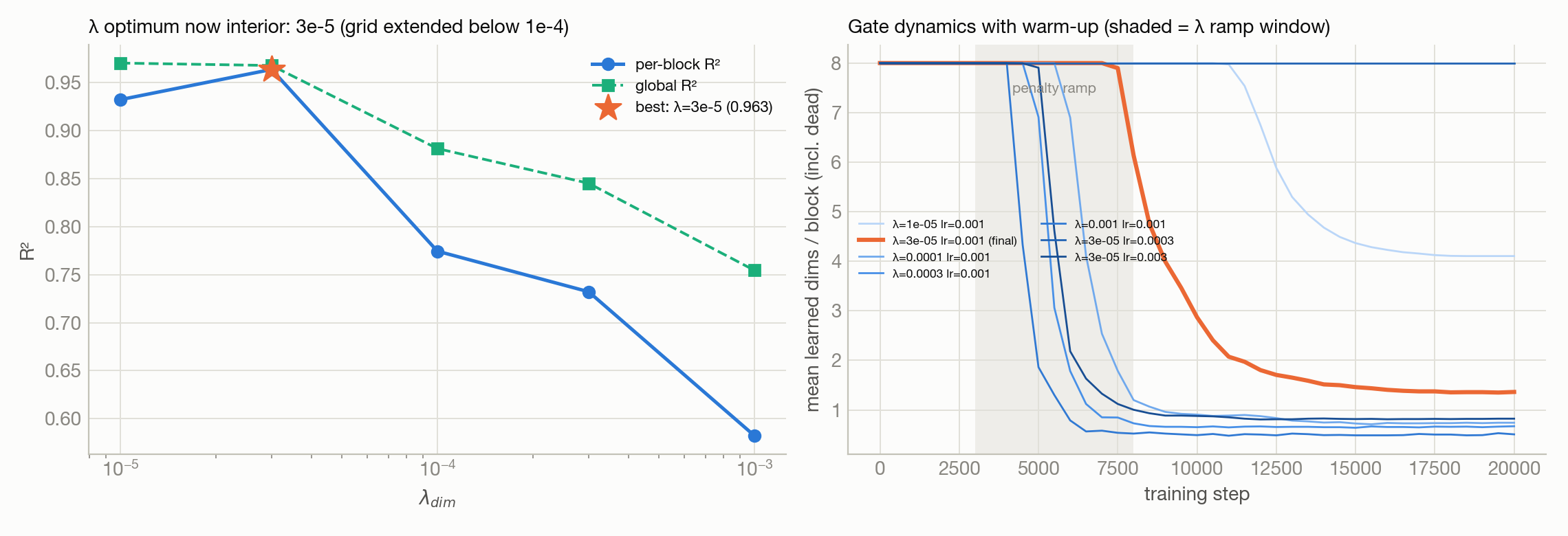
Loss adds λ_dim · (mean dimensions per block). Width 0 kills the block entirely, so one penalty decides both widths and how many concepts exist.
Block Top-K selection is unchanged from Vanilla BSF. A gate warm-up (round 2) holds the penalty at zero for the first 15% of training and ramps it to full by 40%, concepts form before turning dimensions off starts.
Stable rank of each block's held-out contributions is measured after training as an independent probe of geometry; it never enters the objective.

3Result: gates recover the true dimensionality

Toy model: 128 known factors (64 segments + 64 curved manifolds of 7 types) superposed in R¹²⁸, 4 active per sample, no noise; metric = per-block recovery R² against known ground truth.
At strong penalty (λ=10⁻⁴): 144 of 256 blocks turned fully inactive → 112 active vs 128 true factors.
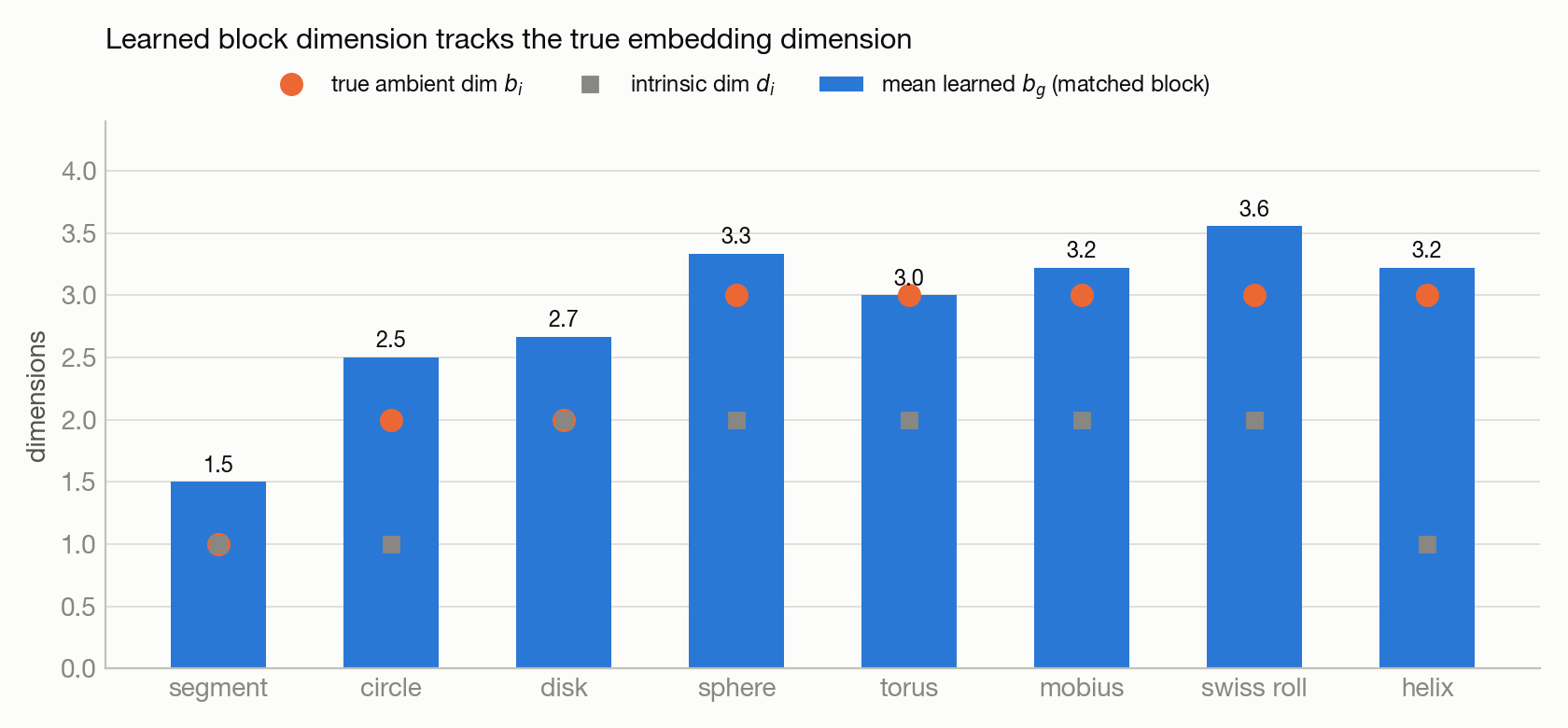
Surviving widths match the truth class by class, segments → 1, circles/disks → 2, all 3-D manifolds → 3 (medians exact for every class).
The helix gets 3 dims: its linear span, not its intrinsic 1-D, exactly what a linear featurizer should discover.
Recovery 0.947 with 9.9 active dims/sample, vs 0.955 at 16 for fixed b=4.

Learned dimension by manifold type — **Figure 1: Learned block width tracks the true embedding dimension.** Strong-penalty run, one bar group per manifold class. blue bars = mean learned width *b_g* of each factor's matched block · orange dots = true ambient dimension *b_i* of the factor's embedding · gray squares = intrinsic manifold dimension. Bars landing on the orange dots is the result.

4Result: adaptive beats every fixed width

With warm-up and the λ grid extended below 10⁻⁴ (optimum moves to an interior 3×10⁻⁵), replicated over four seeds:

Table 1: Per-block recovery on the synthetic toy model, adaptive vs fixed-width and shuffled-width controls (G=256, k=4; ± values over 4 seeds).

Model	Per-block R²	Active dims/sample
Adaptive (learned widths)	0.9626 ± 0.0017	14.7
Vanilla b=3 (best fixed, 4 seeds)	0.9538 ± 0.0066	12
Vanilla b=4 (paper config)	0.9565	16
Vanilla b=2	0.8643	8
Mixed-width (same widths, shuffled)	0.8908	16

+0.009 over the best fixed control ≈ 2.6 standard errors, with ~4× tighter seed variance.
Reproduced end to end: a second independent full run (reduced sweep, same config) lands at 0.963 ± 0.002 again (n=3).
Warm-up also removed round 1's learning-rate fragility (0.947 → 0.963 at the same lr).

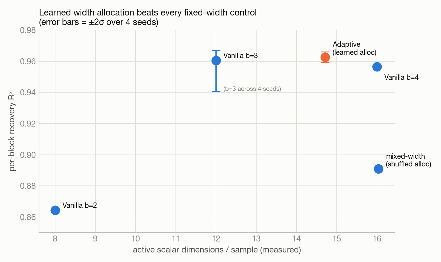
Control comparison scatter — **Figure 2: Learned width-to-concept matching vs fixed and shuffled widths.** Per-block recovery against measured active dimensions per sample. blue points = fixed-width controls (b=2,3,4 and mixed-width) · orange point = adaptive model · error bars = ±2σ over four seeds (adaptive and b=3). The mixed-width point at 16 dims sits 0.07 below the adaptive point.

The decisive control: mixed-width takes the adaptive model's final width histogram, randomly reassigns it across blocks, and freezes it, same total capacity, same width distribution, no learned width-to-concept matching. It falls to 0.891, worse than any uniform width ≥ 3. The value is not "fewer dimensions"; it is which concept gets which width.

5Nuance: gates learn capacity, stable rank measures geometry

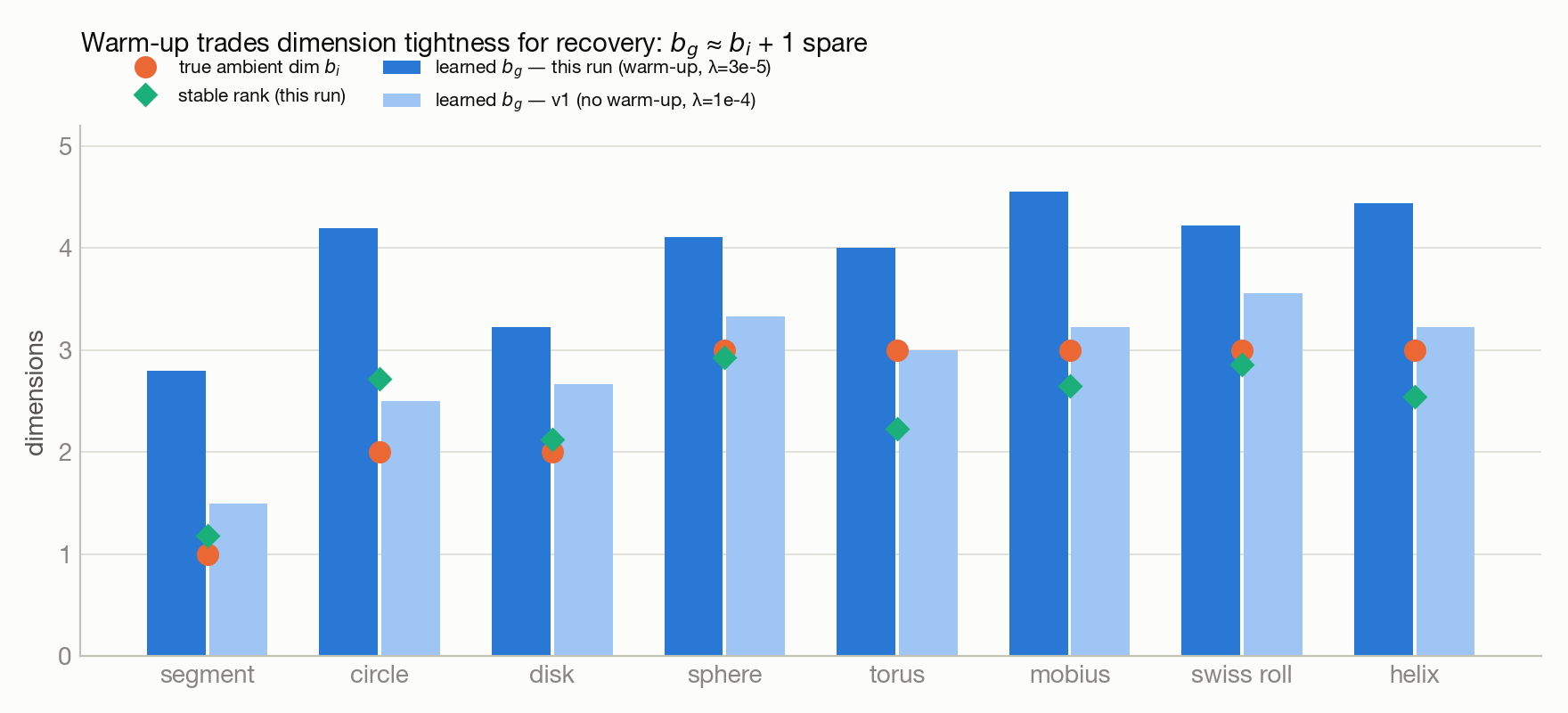
At the recovery-optimal λ the gates keep ~1 spare dimension per concept (segments matched to ≈2.8-wide blocks), but stable rank still tracks the truth (segments 1.2, disks 2.1, spheres 2.9).
Two operating points form a Pareto frontier: exact dimensions @ 0.947 (strong λ, no warm-up) vs +1 spare dim @ 0.963 ± 0.002 (warm-up, gentle λ). A late-ramping λ schedule plausibly reaches both at once (unrun).
Under-turning dimensions off hurts too: at λ=10⁻⁵ nothing is turned off and recovery falls by 0.03, spare dimensions let noise from other concepts in.
Audit of "112 active blocks vs 128 factors": genuine block sharing (15 blocks serve two factors each; the gate-active and fire-active block sets match exactly, 111 = 111). One penalty currently both shrinks widths and deletes blocks, separating those two jobs is the next architectural fix.

**Figure 3: Penalty landscape and gate dynamics.** **Left panel:** per-block R² (blue circles) and global R² (green squares) across λ; orange star = final model at the interior optimum λ=3×10⁻⁵. **Right panel:** mean learned width over training for each λ (blue shades), final model in orange; shaded band = the warm-up ramp window, turning dimensions off begins only inside it and proceeds gradually.

Warm-up run: widths vs truth vs stable rank — **Figure 4: Warm-up trades dimensional tightness for recovery.** dark bars = learned widths, this run (warm-up, λ=3×10⁻⁵) · light bars = round-1 widths (strong penalty) · orange dots = true dimension · green diamonds = stable rank, this run. Learned widths sit ≈1 above truth while stable rank stays on it.

6Real features (DINOv2): worst reconstruction, best probe

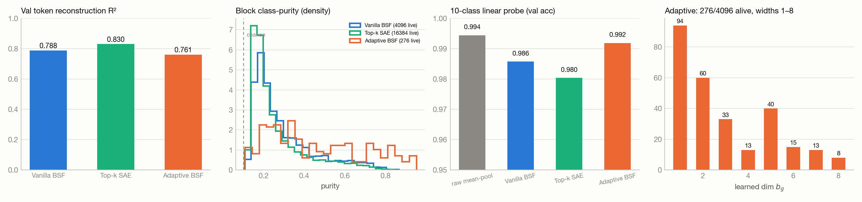
Table 2: DINOv2 patch activations: reconstruction, surviving blocks, and 10-class linear-probe accuracy (Imagenette).

Model	Recon R²	Active blocks	Probe acc
raw features (baseline)	n/a	n/a	0.994
Top-K SAE (16,384 atoms)	0.830	16384	0.980
Vanilla BSF (G=4096, b=4)	0.788	4096	0.986
Adaptive BSF (b_max=8)	0.761	276	0.992

Setup: 1.2M DINOv2-base patch tokens from Imagenette; probe = 10-class linear readout on pooled block codes.
Reconstruction vs usefulness: the SAE reconstructs best and probes worst; adaptive reconstructs worst and probes best with 15× fewer active features. Without ever seeing labels, the penalty behaves like a filter that keeps task-useful structure, the variance it throws away is disproportionately noise.
Real-feature widths are heavy-tailed: mostly 1–2 dims, plus a minority of genuinely 5–8-dimensional concepts.
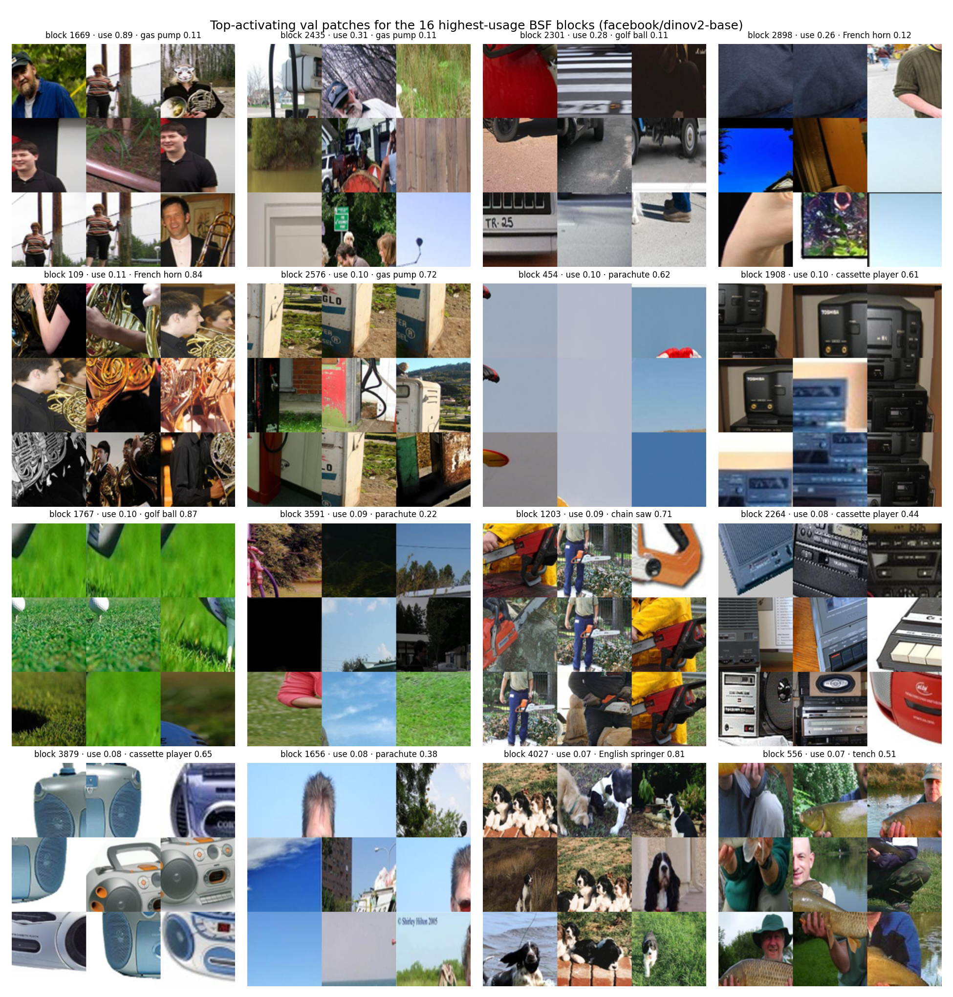
Correction we caught ourselves on: adaptive's higher average purity (0.46 vs 0.29) is a selection effect among the surviving blocks, Vanilla's top-276 blocks by usage are equally pure (0.460). Gates auto-select a compact, pure subset; they do not create purer blocks.

DINO quantitative overview — **Figure 5: DINOv2 quantitative overview.** Panels, left to right: (a) held-out token reconstruction R² per model · (b) class-purity distributions over active blocks (blue = Vanilla, green = SAE, orange = Adaptive; dashed line = 10-class chance) · (c) linear-probe accuracy vs the raw-feature baseline (gray) · (d) adaptive width histogram, 276 survivors of 4,096, widths 1–8.

Top-activating patches per block — **Figure 6: Blocks line up with concepts you can point to.** Each 3×3 grid = the top-activating validation patches of one high-usage BSF block; the header gives block id, fire rate, top class and purity. high-purity blocks are concepts you can point to, French horn (0.84), golf-ball-on-grass (0.87), chainsaw (0.71), stereo equipment, springer spaniels (0.81), tench-with-angler. The busiest blocks (top row) are generic people/sky/ground textures with low purity, a usage↔purity tradeoff.

7Limits and what's next

Single dataset seed; single-seed gaps under 0.01 are noise (headline comparisons are 4-seed).
DINO run used DINOv2 (v3 weights gated), a toy-tuned λ with no sweep, and 10 coarse labels, needs a λ sweep, capacity-matched re-run, seeds, and attribute-level evaluation (TAPAScore/synCUB).
SASA (2026) concurrently learns per-group rank via a nuclear norm, adjacent territory. Distinct here: hard prefix gates, the shuffled-width causal control, and the capacity-vs-geometry separation.
Scope of the win: at matched dictionary size (G=256, k=4) adaptive beats all three author models (Vanilla 0.956, Group-Lasso 0.946, Grassmannian 0.866). The authors' Vanilla at G=512 reaches 0.972; adaptive at G=512 is untested.
Two further extensions ran and failed, usefully. Matching-pursuit block selection: better reconstruction (global 0.993 vs 0.969) but worse factor recovery (0.899 vs 0.955), and the correlated-subspace variant barely hurt Vanilla (0.947 at rho 0.6). Atlas multi-chart blocks on the nonlinear-span toy model: 0.685, below plain b=4 (0.700) and b=16 (0.724).
Still queued: late-λ ramp (both ends of the Pareto frontier at once); separate block-existence vs width penalties.

8Sources

Fel et al. Structuring Sparsity: Block-Sparse Featurizers Capture Visual Concept Manifolds. arXiv:2606.25234 · official code
Costa et al. From Flat to Hierarchical: Extracting Sparse Representations with Matching Pursuit. arXiv:2506.03093
Dalili & Mahdavi. Subspace-Aware Sparse Autoencoders (SASA). arXiv:2606.06333
Schonsheck et al. Chart Auto-Encoders for Manifold Structured Data. arXiv:1912.10094
SoftSAE: Dynamic Top-K Selection. arXiv:2605.06610 · SpaDE. arXiv:2503.01822
TAPAScore / synCUB concept-annotation toy model. arXiv:2606.24716
Oquab et al. DINOv2. arXiv:2304.07193

All numbers from self-contained Colab notebooks with cached runs, recorded deviations, and exported archives

Adaptive-Dimensional Block-Sparse Featurizers:Learning How Wide Each Concept Should Be