Block-Sparse Featurizers Beyond Fixed Widths:
Learned Allocation, Label-Guided Organization, and What Reconstruction Misses

Edward Lu

Research notes · August 2026 · not peer reviewed

Abstract Block-sparse featurizers (Fel et al., 2026) hold multi-dimensional concepts together by making sparsity act between blocks rather than between rank-one atoms — but every block gets the same hand-chosen width, block↔concept assignment is left to chance, and quality is judged by reconstruction. We relax all three, one controlled experiment at a time. (1) Learned widths: ordered prefix gates let each block choose its own dimension under a dimension-use penalty; on the paper's synthetic benchmark the gates recover how many concepts exist and how wide each is, beat every fixed width across seeds, and a shuffled-width control shows the win is which concept gets which width. On DINOv2 the same penalty keeps 276 of 4,096 blocks yet nearly matches a raw-feature probe. (2) Weak semantic alignment: harmful on the toy (assignment was already one-to-one), as predicted it reverses on real features — 1% of ADE20K labels doubles block purity and cuts class shattering from 626 to 173 blocks at matched reconstruction. (3) Fidelity: across the toy, DINOv2, and GPT-2, the best-reconstructing featurizer is repeatedly not the most faithful one — splice CE and probes dissociate from R², arguing reconstruction is the wrong objective to trust. Negative results (coordinate steering, matching-pursuit selection, multi-chart decoders) are reported with their controls.

1Three questions, one framework

BSF's block prior fixes the shattering that flat SAEs inflict on curved concept manifolds, but leaves three choices to the practitioner: block width b (one global sweep), block identity (unsupervised), and the training objective (reconstruction MSE with architectural Top-K — Eq. 4 of the paper, which all models here implement verbatim from the official code).
We ask: can width be learned per concept; can a few labels organize which block a concept lands in; and does reconstruction quality actually track how much of the computation a featurizer preserves?
Testbeds: the paper's own controlled toy model (128 known factors — 64 segments, 64 curved manifolds — superposed in R¹²⁸, ground-truth per-block recovery R²), DINOv2-base patch tokens (Imagenette; ADE20K for labels), and GPT-2 Medium residual streams. All runs seeded, cached, and exported with recorded deviations.

2Learned widths: ordered prefix gates

Each block gets a maximum width b_max and gate logits θ; the soft mask is a cumulative product of sigmoids, so the hard mask is always a prefix — 1,1,1,0,0,0 → width 3. The forward pass uses the hard {0,1} mask with a straight-through gradient: pruned dimensions are exactly inactive.
The loss adds λ_dim · (mean dimensions per block). Width 0 deletes the block, so one penalty decides both widths and the number of live concepts. Block Top-K is untouched. A warm-up holds the penalty at zero for the first 15% of training so concepts form before pruning starts.
At strong penalty the gates recover the truth class by class: segments → 1, circles/disks → 2, 3-D manifolds → 3 (medians exact), and 144 of 256 blocks die — 112 survivors for 128 true factors. The helix gets its linear span (3), not its intrinsic dimension (1) — exactly what a linear featurizer should discover.

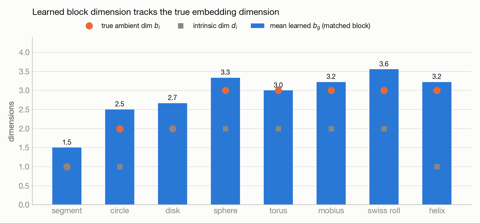
Learned dimension by manifold type — **Figure 1: Learned block width tracks the true embedding dimension.** blue bars = mean learned width of each factor's matched block · orange dots = true ambient dimension · gray squares = intrinsic dimension. Bars landing on the orange dots is the result.

Table 1: Per-block recovery on the toy model (G=256, k=4; ± over 4 seeds). Warm-up run, λ grid extended to its interior optimum 3×10⁻⁵.

Model	Per-block R²	Active dims/sample
Adaptive (learned widths)	0.9626 ± 0.0017	14.7
Vanilla b=3 (best fixed, 4 seeds)	0.9538 ± 0.0066	12
Vanilla b=4 (paper config)	0.9565	16
Vanilla b=2	0.8643	8
Mixed-width (same widths, shuffled)	0.8908	16

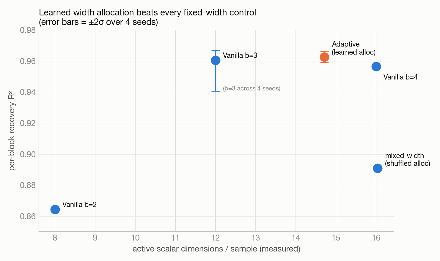
Control comparison — **Figure 2: Learned width-to-concept matching beats fixed and shuffled widths.** blue = fixed-width controls · orange = adaptive · error bars ±2σ over four seeds.

The decisive control: mixed-width takes the adaptive model's final width histogram, reassigns it randomly across blocks, and freezes it — same capacity, same distribution, no learned matching. It falls to 0.891, worse than any uniform width ≥ 3. The value is not "fewer dimensions"; it is which concept gets which width. The gain (+0.009 over the best fixed control, ≈2.6 standard errors, ~4× tighter seed variance) reproduced in a second independent full run. Nuance: at the recovery-optimal λ the gates keep ≈1 spare dimension per concept while stable rank still sits on the truth (segments 1.2, disks 2.1, spheres 2.9) — gates learn capacity; stable rank measures geometry; the strong-λ point (exact widths, R² 0.947) and the warm-up point (spare dim, 0.963) form a Pareto frontier a late-ramping schedule might close.

3Learned widths on real features: an unsupervised filter

Table 2: DINOv2 patch activations (Imagenette): reconstruction, surviving blocks, 10-class linear probe.

Model	Recon R²	Active blocks	Probe acc
raw features (baseline)	n/a	n/a	0.994
Top-K SAE (16,384 atoms)	0.830	16384	0.980
Vanilla BSF (G=4096, b=4)	0.788	4096	0.986
Adaptive BSF (b_max=8)	0.761	276	0.992

The penalty keeps 276 of 4,096 blocks and still nearly matches the raw-feature probe with 15× fewer active features — without ever seeing a label, it behaves like a filter that keeps task-useful structure. Real-feature widths are heavy-tailed: mostly 1–2 dims plus a minority of genuinely 5–8-dimensional concepts.
Correction we caught ourselves on: adaptive's higher average purity (0.46 vs 0.29) is a survivor-selection effect — Vanilla's top-276 blocks by usage are equally pure (0.460). Gates auto-select a compact, pure subset; they do not create purer blocks.

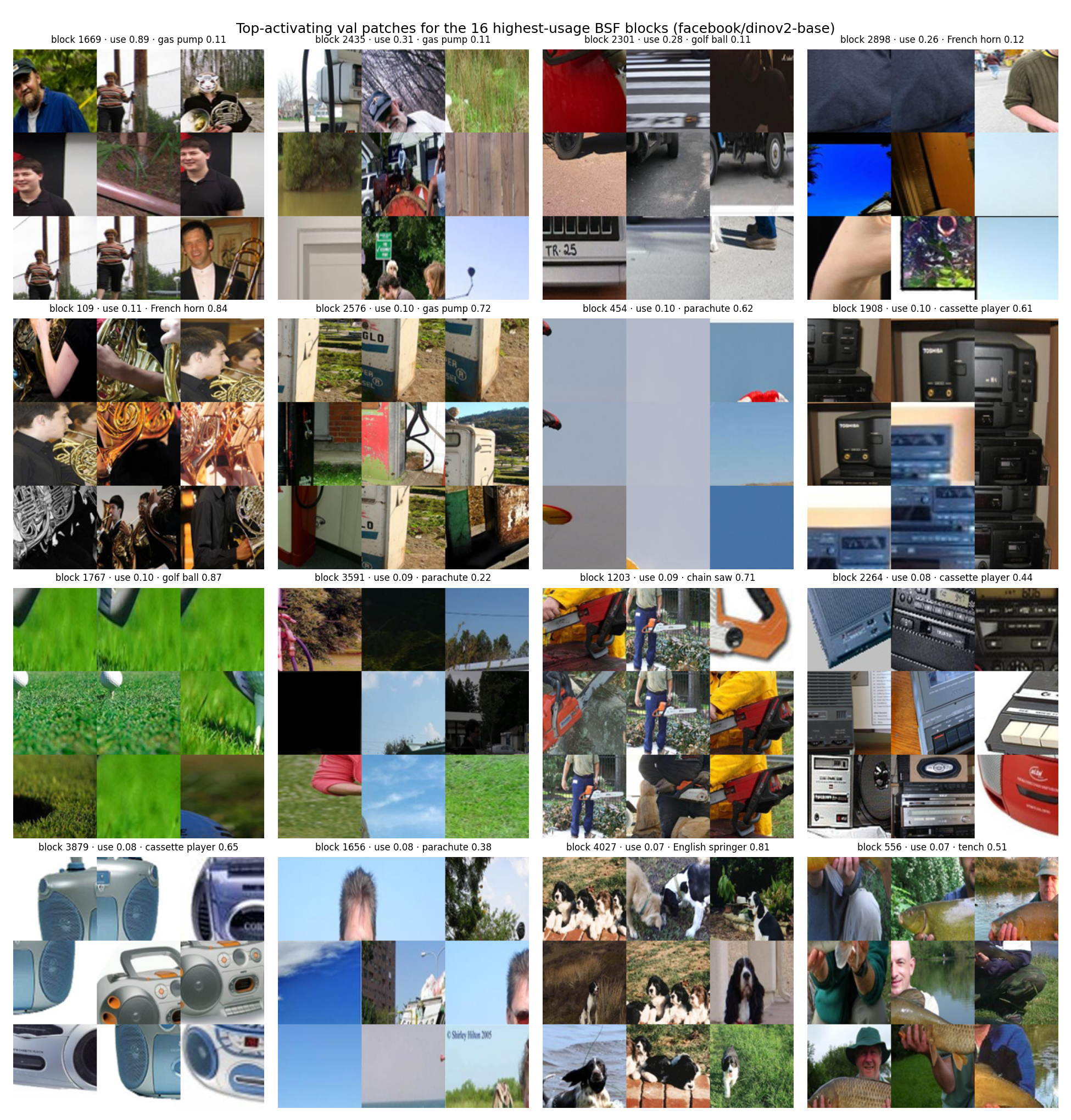
Top-activating patches per block — **Figure 3: Blocks line up with concepts you can point to.** Each 3×3 grid = top-activating validation patches of one high-usage block (id, fire rate, top class, purity in the header). French horn (0.84), golf-ball-on-grass (0.87), chainsaw (0.71), stereo equipment, springer spaniels (0.81); the busiest blocks are generic people/sky/ground textures — a usage↔purity tradeoff.

4Semantic alignment: a toy failure that predicted a real-data success

On the toy model, weakly supervising block identity was strictly harmful at every labeled fraction: the unsupervised assignment was already one-to-one, so labels only perturbed training. Prediction from that null: supervision helps exactly when assignment is underdetermined — i.e. on real, polysemantic features.
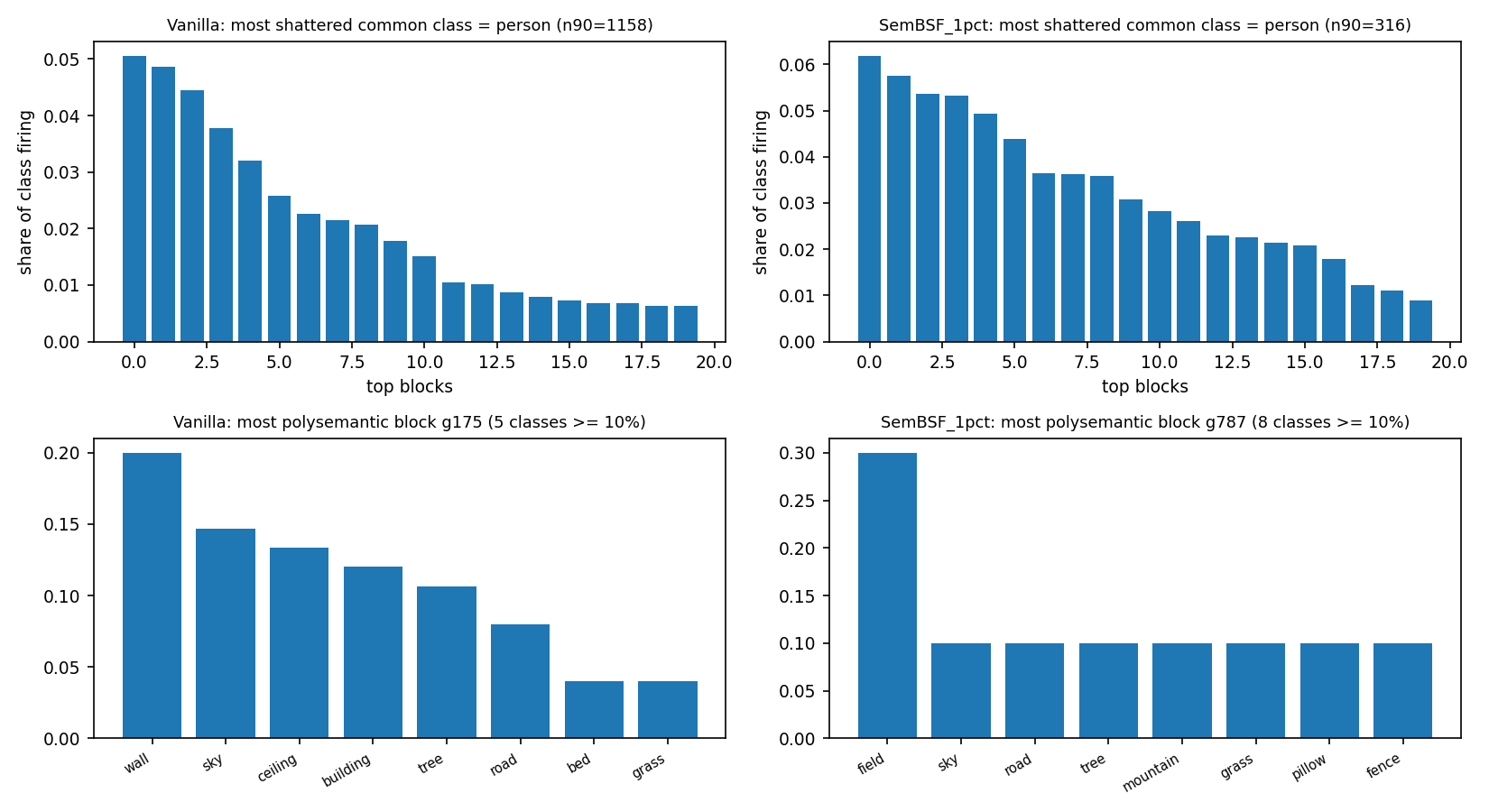
Test: DINOv2 tokens with ADE20K segmentation classes as weak labels. For labeled tokens, a supervised-contrastive pull (SupCon) on normalized pre-TopK block-support vectors — same class, different image → similar block usage; no class→block assignment anywhere. The term is scaled by the reconstruction loss and warmup-gated (both lessons from the toy failure). Fractions 0/1/5/10% of images.

Table 3: Semantic supervision on DINOv2 + ADE20K. Purity = mean class purity over live blocks; n90 = blocks covering 90% of a class's firing (common classes); entropy = class→block firing entropy.

Run	Global R²	Live blocks	Purity	n90	Entropy
Vanilla BSF	0.774	4096	0.252	626	5.69
Sem 0% (protocol twin)	0.774	4096	0.252	617	5.67
Sem 1%	0.742	3716	0.541	173	4.57
Sem 5%	0.743	3285	0.576	87	4.09
Sem 10%	0.750	3169	0.586	97	4.18

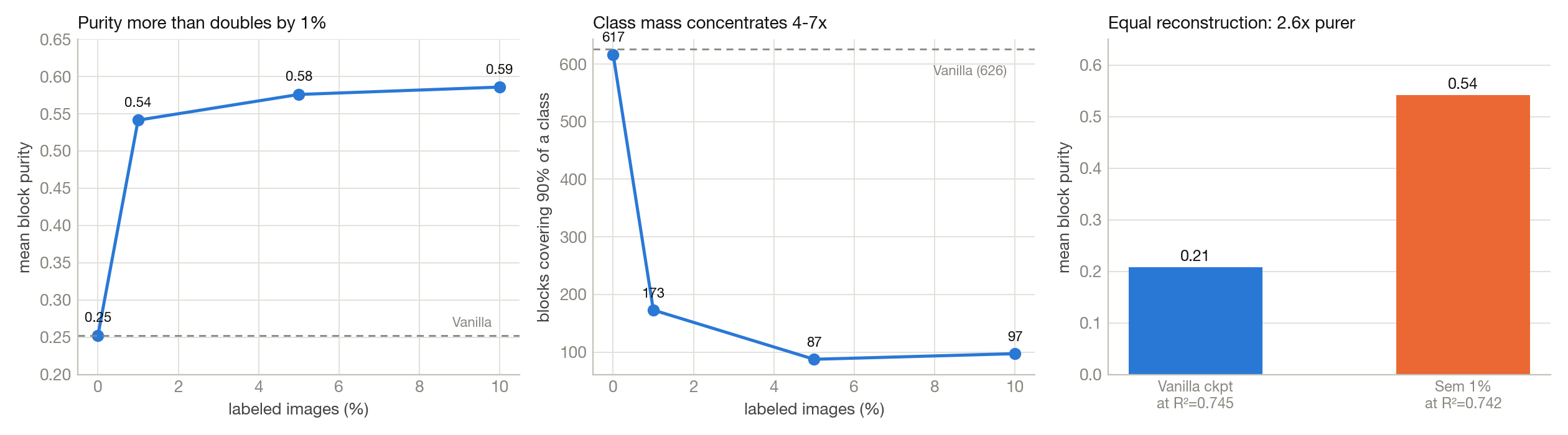
Purity and concentration vs labeled fraction — **Figure 4: One percent of labels reorganizes the dictionary.** **Left:** mean block purity vs labeled fraction (dashed = Vanilla). **Middle:** blocks needed for 90% of a class's mass. **Right:** at equal reconstruction (R²≈0.74) the nearest Vanilla checkpoint reaches purity 0.21 vs 0.54 for Sem 1%.

The decisive control: semantic runs reconstruct slightly worse (−0.02 to −0.03 R²), so the purity gain could be an earlier point on the Vanilla trajectory. Scoring the Vanilla checkpoint of matched R² (step 2,500, R²=0.745): purity 0.209 and n90 965, vs 0.541 and 173 for Sem 1%. At equal reconstruction the semantic model is ≈2.6× purer and ≈5.6× more concentrated; the 0% twin lands on Vanilla within the pre-measured seed-noise yardstick (Δpurity 0.003), so the procedure alone does nothing. Costs stay real and reported: high-traffic generic blocks stay generic (usage-weighted purity is flat), and global class–block NMI degrades past 1% — supervision organizes the tail, not the busy head, and label appetite saturates by 5%.

Shattering before and after — **Figure 5: What supervision changes.** The most shattered common class (person) needs 1,158 blocks for 90% of its mass under Vanilla, 316 under Sem 1%; the same small block set carries a class across very different images.

5Fidelity: reconstruction is the wrong thing to trust

On GPT-2 Medium (layer 12, ~1M tokens over prose/reviews/code), each featurizer's reconstruction is spliced into the forward pass and the damage read off next-token cross-entropy (clean 3.31, zero-ablation 14.95):

Table 4: Reconstruction vs downstream fidelity under CE-splice, matched dictionary size (~16.8M params).

Featurizer	Recon R²	CE Δ vs clean	Frac recovered
Top-K SAE (8192, k=32)	0.732	1.154	0.901
Vanilla BSF b=4	0.664	0.859	0.926
Wide-block BSF (b=8)	0.706	0.673	0.942

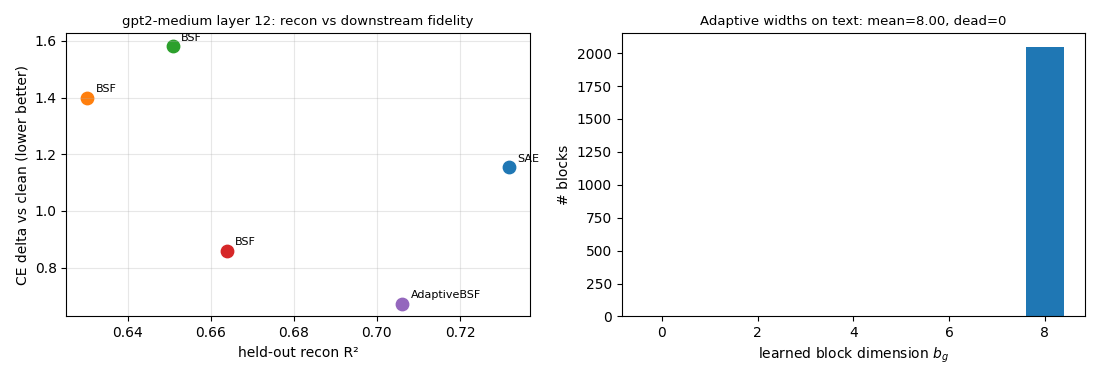
Recon vs CE delta — **Figure 6: The best-reconstructing featurizer damages the model most.** **Left:** reconstruction R² vs splice damage per featurizer — the SAE sits right and high, block models left and low. **Right:** the "adaptive" row's gates never pruned on text (all widths at 8), so it is reported as what it is: a wide-block Vanilla; learned allocation on language still needs its own λ sweep.

This is the series' most consistent regularity, seen on three unrelated surfaces: the GPT-2 SAE reconstructs best and splices worst; the DINOv2 adaptive model reconstructs worst and probes best (Table 2); and on the toy, matching-pursuit selection lifted global reconstruction to 0.993 while dropping factor recovery to 0.899. What a featurizer keeps matters more than how much it keeps — evaluation should weight splice/probe fidelity and recovery over R².

6What did not work

Within-block coordinate steering (GPT-2): a clean null. With common-random-number generation (identical sampling seed per prompt across conditions), discovery/steering data disjoint, and five matched-norm controls, editing a single block coordinate moved the dominant attribute no more than a random residual direction (0.594 vs 0.642) — though it cost the least fluency and preserved the concept best among out-of-block edits. Block identity probes semantically (source acc up to 0.99), but the shuffled-feature floor matches it almost everywhere; exactly one of eight blocks showed genuine coordinate structure. At this scale, blocks are semantic identity units with mostly unstructured interiors.
Matching-pursuit block selection: residual-guided greedy selection (after MP-SAE) reconstructed better and recovered factors worse in both the incoherent and correlated toy settings — the greedy residual objective blurs factor attribution on additive superpositions.
Atlas multi-chart blocks: on a purpose-built nonlinear-span toy variant (curved manifolds sinusoidally lifted so intrinsic dim ≪ linear span), 4 charts × 4 dims scored 0.685 — below plain b=4 (0.700) and wide b=16 (0.724). The benchmark itself works (b=4 collapses exactly where designed) and is the right arena for future nonlinear decoders; this decoder wasn't it.
Toy semantic alignment: harmful at every fraction — the failure that correctly predicted Section 4's success condition.

7Limits and what's next

Single dataset seed throughout; headline comparisons are 4-seed, single-seed gaps under ~0.01 are noise.
Vision runs used DINOv2 and the LLM run GPT-2 Medium — the gated DINOv3/Gemma-2-2B targets (and the Gemma Scope anchor) need a working HF token; both fallbacks are recorded in the archives.
SASA (2026) concurrently learns per-group rank via a nuclear norm — adjacent territory. Distinct here: hard prefix gates, the shuffled-width causal control, the capacity-vs-geometry separation, and the label-guided organization result.
Queued: late-λ ramp (exact widths and peak recovery), separate block-existence vs width penalties, a text-scale λ sweep, coordinate-structured-block search (select by probe-minus-shuffled gap), and attribute-level evaluation (TAPAScore/synCUB) in place of coarse labels.

8Sources

Fel et al. Structuring Sparsity: Block-Sparse Featurizers Capture Visual Concept Manifolds. arXiv:2606.25234 · official code
Khosla et al. Supervised Contrastive Learning. arXiv:2004.11362
Gao et al. Scaling and Evaluating Sparse Autoencoders (CE-splice fidelity metric). arXiv:2406.04093
Costa et al. From Flat to Hierarchical: Extracting Sparse Representations with Matching Pursuit. arXiv:2506.03093
Dalili & Mahdavi. Subspace-Aware Sparse Autoencoders (SASA). arXiv:2606.06333
Schonsheck et al. Chart Auto-Encoders for Manifold Structured Data. arXiv:1912.10094
Lieberum et al. Gemma Scope. arXiv:2408.05147 · Oquab et al. DINOv2. arXiv:2304.07193 · TAPAScore / synCUB. arXiv:2606.24716

All numbers from self-contained Colab notebooks with cached runs, recorded deviations, and exported archives

Block-Sparse Featurizers Beyond Fixed Widths:Learned Allocation, Label-Guided Organization, and What Reconstruction Misses